Quick Model Building
Building a quick Michaelis-Menten reaction using COPASI’s automatisms. Working with reaction equations automatically creates required entities the same way the COPASI GUI does.
newModel()
#> # A COPASI model reference:
#> Model name: "New Model"
#> Number of compartments: 0
#> Number of species: 0
#> Number of reactions: 0
newReaction("a = b", fun = "Reversible Michaelis-Menten")
#> [1] "(a = b)"
getSpecies()
#> # A tibble: 2 × 13
#> key name compa…¹ type unit initi…² initi…³ conce…⁴ number rate numbe…⁵
#> <chr> <chr> <chr> <chr> <chr> <dbl> <dbl> <dbl> <dbl> <dbl> <dbl>
#> 1 a{comp… a compar… reac… mol/l 1 6.02e23 NaN NaN 0 0
#> 2 b{comp… b compar… reac… mol/l 1 6.02e23 NaN NaN 0 0
#> # … with 2 more variables: initial_expression <chr>, expression <chr>, and
#> # abbreviated variable names ¹compartment, ²initial_concentration,
#> # ³initial_number, ⁴concentration, ⁵number_rate
getReactions()
#> # A tibble: 1 × 6
#> key name reaction rate_law flux numbe…¹
#> <chr> <chr> <chr> <chr> <dbl> <dbl>
#> 1 (a = b) a = b a = b FunctionDB.Functions[Reversible Michaeli… 0 0
#> # … with abbreviated variable name ¹number_flux
getParameters()
#> # A tibble: 4 × 5
#> key name reaction value mapping
#> <chr> <chr> <chr> <dbl> <chr>
#> 1 (a = b).Kms Kms a = b 0.1 NA
#> 2 (a = b).Kmp Kmp a = b 0.1 NA
#> 3 (a = b).Vf Vf a = b 0.1 NA
#> 4 (a = b).Vr Vr a = b 0.1 NA
unloadModel()More Detail
Getting more detail in can be helpful. Here we create a global
quantity “substrate concentration” which applies a fixed value to
species “a”. This is achieved by assigning the Value
reference of the global quantity to species “a”.
newModel()
#> # A COPASI model reference:
#> Model name: "New Model"
#> Number of compartments: 0
#> Number of species: 0
#> Number of reactions: 0
subs_quant <- newGlobalQuantity("substrate concentration", initial_value = 10)
subs_value <- quantity(subs_quant, reference = "Value")
subs_value
#> [1] "{Values[substrate concentration]}"
newSpecies("a", type = "assignment", expression = subs_value)
#> Warning: No compartment exists. Created default compartment.
#> [1] "a{compartment}"
newReaction("a = b", fun = "Reversible Michaelis-Menten")
#> [1] "(a = b)"
getGlobalQuantities()
#> # A tibble: 1 × 9
#> key name type unit initi…¹ value rate initi…² expre…³
#> <chr> <chr> <chr> <chr> <dbl> <dbl> <dbl> <chr> <chr>
#> 1 Values[substrate concen… subs… fixed "" 10 NaN 0 "" ""
#> # … with abbreviated variable names ¹initial_value, ²initial_expression,
#> # ³expression
getSpecies()
#> # A tibble: 2 × 13
#> key name compa…¹ type unit initi…² initi…³ conce…⁴ number rate numbe…⁵
#> <chr> <chr> <chr> <chr> <chr> <dbl> <dbl> <dbl> <dbl> <dbl> <dbl>
#> 1 a{comp… a compar… assi… mol/l 10 6.02e24 NaN NaN NaN NaN
#> 2 b{comp… b compar… reac… mol/l 1 6.02e23 NaN NaN 0 0
#> # … with 2 more variables: initial_expression <chr>, expression <chr>, and
#> # abbreviated variable names ¹compartment, ²initial_concentration,
#> # ³initial_number, ⁴concentration, ⁵number_rate
getReactions()
#> # A tibble: 1 × 6
#> key name reaction rate_law flux numbe…¹
#> <chr> <chr> <chr> <chr> <dbl> <dbl>
#> 1 (a = b) a = b a = b FunctionDB.Functions[Reversible Michaeli… 0 0
#> # … with abbreviated variable name ¹number_flux
getParameters()
#> # A tibble: 4 × 5
#> key name reaction value mapping
#> <chr> <chr> <chr> <dbl> <chr>
#> 1 (a = b).Kms Kms a = b 0.1 NA
#> 2 (a = b).Kmp Kmp a = b 0.1 NA
#> 3 (a = b).Vf Vf a = b 0.1 NA
#> 4 (a = b).Vr Vr a = b 0.1 NA
timecourse <- runTimeCourse(1000)
autoplot.copasi_ts(timecourse)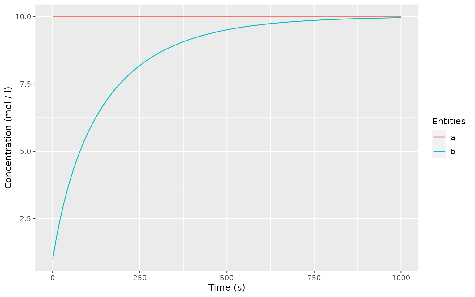
Defining Reaction Kinetics Manually
In previous examples, we used the predefined “Reversible Michaelis-Menten” kinetic functions. In this example we create an equivalent function manually to achieve the same result.
newModel()
#> # A COPASI model reference:
#> Model name: "New Model"
#> Number of compartments: 0
#> Number of species: 0
#> Number of reactions: 0

newCompartment("compartment")
#> [1] "Compartments[compartment]"
newSpecies("a", type = "fixed", initial_concentration = 10)
#> [1] "a{compartment}"
newSpecies("b")
#> [1] "b{compartment}"
newKineticFunction(
  "manual MM",
  "((Vf * substrate) / Kms - Vr * product / Kmp) / (1 + substrate / Kms + product / Kms)",
  parameters = list(substrate = "substrate", product = "product")
)
#> [1] "FunctionDB.Functions[manual MM]"
newReaction(
  "a = b",
  fun = "manual MM",
  mapping = list(
    substrate = "a",
    product = "b",
    Vf = 0.1,
    Kms = 0.1,
    Vr = 0.1,
    Kmp = 0.1
  )
)
#> [1] "(a = b)"

timecourse <- runTimeCourse(1000)

autoplot.copasi_ts(timecourse)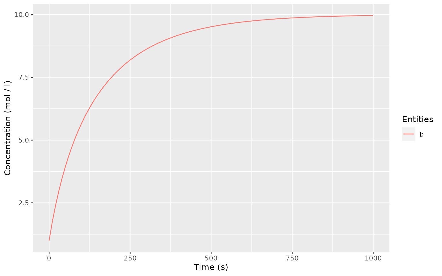
Quantities as Proxy for Time Course Output
The runTimeCourse function only returns data for actual
defined entities of the model. Auxiliarry information like reaction
rates can be missing and needs to be added via global quantity
assignments. This example creates a global quantity “reaction rate” to
generate data for the main reaction’s flux.
newModel()
#> # A COPASI model reference:
#> Model name: "New Model"
#> Number of compartments: 0
#> Number of species: 0
#> Number of reactions: 0

subs_quant <- newGlobalQuantity("substrate concentration", initial_value = 10)
subs_value <- quantity(subs_quant, reference = "Value")

newSpecies("a", type = "assignment", expression = subs_value)
#> Warning: No compartment exists. Created default compartment.
#> [1] "a{compartment}"
newReaction("a = b", fun = "Reversible Michaelis-Menten")
#> [1] "(a = b)"

runTC(1000)$result
#> # A tibble: 101 × 3
#>     Time     b     a
#>    <dbl> <dbl> <dbl>
#>  1     0  1       10
#>  2    10  1.75    10
#>  3    20  2.40    10
#>  4    30  2.97    10
#>  5    40  3.48    10
#>  6    50  3.94    10
#>  7    60  4.35    10
#>  8    70  4.72    10
#>  9    80  5.06    10
#> 10    90  5.37    10
#> # … with 91 more rows

newGlobalQuantity(
  "reaction rate",
  type = "assignment",
  expression = reaction("a = b", reference = "Flux")
)
#> [1] "Values[reaction rate]"

runTimeCourse(1000)$result
#> # A tibble: 101 × 4
#>     Time     b     a `Values[reaction rate]`
#>    <dbl> <dbl> <dbl>                   <dbl>
#>  1     0  1       10                  0.0811
#>  2    10  1.75    10                  0.0696
#>  3    20  2.40    10                  0.0608
#>  4    30  2.97    10                  0.0538
#>  5    40  3.48    10                  0.0480
#>  6    50  3.94    10                  0.0432
#>  7    60  4.35    10                  0.0391
#>  8    70  4.72    10                  0.0356
#>  9    80  5.06    10                  0.0326
#> 10    90  5.37    10                  0.0299
#> # … with 91 more rows

unloadModel()