Michaelis Menten Kinetics
Johanna Daas, Jonas Förster and Jürgen Pahle
Setup
The code in this teaching document uses the R packages CoRC and tidyverse. Make sure they are installed before beginning. If you have not yet downloaded CoRC, take a look at the tab Download.
Code
library(CoRC)
library(tidyverse)
Download
# install tidyverse
install.packages("tidyverse")

# install CoRC from GitHub
install.packages("remotes")
remotes::install_github("jpahle/CoRC")
Introduction
Michaelis-Menten-Kinetics, introduced by Leonor Michaelis and Maud Menten1 is a popular model of enzyme kinetics.
If you have a substrate \(S\) and product \(P\) and the reaction is catalyzed by enzyme \(E\), you can use Michaelis-Menten-Kinetics to describe this process. The rate of formation of the product (\(v\)) is given by
\[ v = \frac{V_{max} * [S]}{K_M + [S]} \]
with \(V_{max}\) the maximum rate of product formation (at saturating substrate concentration) and \(K_M\) the value of the Michaelis-Constant.
Derivation
Michaelis-Menten kinetics follow the assumption that enzyme-catalyzed reactions follow a two step process
\[ S + E \rightleftharpoons SE \rightarrow E + P \]
where the substrate and the enzyme reversibly form a complex \(SE\) (with parameters \(k_f\) and \(k_r\) for forward and reverse reactions) which then catalyses the formation of the product and the release of the enzyme (with reaction parameter \(k_{cat}\)).
In this model, all our reaction follow Mass-action kinetics where the reaction rate is proportional to the concentration of the substrates.
We can denote our reaction rates for the two reactions as follows:
1.) \(k_f*([S]+[E]) - k_r*[SE]\)
2.) \(k_{cat}*[SE]\)
We can form 4 differential equations to describe the change of our species concentrations over time:
\[\frac{d[S]}{dt} = - k_f[S][E] + k_r[SE]\] \[\frac{d[E]}{dt} = -k_f[S][E] + k_r[SE] + k_{cat}[SE]\] \[\frac{d[ES]}{dt} = k_f[S][E] - k_r[SE] - k_{cat}[SE] \] \[\frac{d[P]}{dt} = k_{cat}[SE]\]
Another important assumption is, that the concentration of the substrate is much higher than the concentration of the enzyme.
Model in CoRC
We can visualise this model using CoRC:
First, we have to create a new model
newModel()
#> # A COPASI model reference:
#> Model name: "New Model"
#> Number of compartments: 0
#> Number of species: 0
#> Number of reactions: 0
setModelName("Manual Michaelis Menten")
Next, we can put in our reactions. Species that are called in the
reaction creation and are not part of the model yet, will be added
automatically. We can denote reversible reactions with an =
sign, and non-reversible reactions with an arrow ->.
Hint: Make sure that all species and operators are separated by a space,
otherwise CoRC will not see them as distinct
species/things.
newReaction("S + E = SE")
#> [1] "(S + E = SE)"
newReaction("SE -> P + E")
#> [1] "(SE -> P + E)"
We will now take a look at the species and the reactions in our model.
getSpecies()
#> # A tibble: 4 × 13
#>   key             name  compartment type   unit  initial_concent… initial_number
#>   <chr>           <chr> <chr>       <chr>  <chr>            <dbl>          <dbl>
#> 1 E{compartment}  E     compartment react… mol/l                1        6.02e23
#> 2 S{compartment}  S     compartment react… mol/l                1        6.02e23
#> 3 SE{compartment} SE    compartment react… mol/l                1        6.02e23
#> 4 P{compartment}  P     compartment react… mol/l                1        6.02e23
#> # … with 6 more variables: concentration <dbl>, number <dbl>, rate <dbl>,
#> #   number_rate <dbl>, initial_expression <chr>, expression <chr>
getReactions()
#> # A tibble: 2 × 6
#>   key           name        reaction    rate_law                flux number_flux
#>   <chr>         <chr>       <chr>       <chr>                  <dbl>       <dbl>
#> 1 (S + E = SE)  S + E = SE  S + E = SE  FunctionDB.Functions[…     0           0
#> 2 (SE -> P + E) SE -> P + E SE -> P + E FunctionDB.Functions[…     0           0
getReactions()$rate_law
#> [1] "FunctionDB.Functions[Mass action (reversible)]"
#> [2] "FunctionDB.Functions[Mass action (irreversible)]"
As you can see, the species in the model all start with a concentration of 1. This obviously does not make sense for our model, because at the beginning, we don’t want there to be any complex or product. Also, we will need to make sure that there is a lot more substrate than complex (as this is one of the assumptions). The reactions look fine; the rate law is automatically set to Mass Action Kinetics, which is (as you will see below) needed for Michaelis-Menten Kinetics.
setSpecies(key = species(), initial_concentration = c(1,20,0,0))Now, we want to know how our model behaves. For this, we will
simulate how our species interact with each other in a time
course. The runTimeCourse() command gives us a list
with a lot of different aspects, but for now, only the “result” section
is interesting to us.
timecourse <- runTimeCourse(duration = 1000, dt = 1)$resultWe will now need to reshape the data to make it printable with ggplot.
#Reshape
timecourse <- pivot_longer(timecourse, -Time, values_to = "Concentration", names_to = "Species")

timecourse
#> # A tibble: 4,004 × 3
#>     Time Species Concentration
#>    <dbl> <chr>           <dbl>
#>  1     0 E              1
#>  2     0 S             20
#>  3     0 SE             0
#>  4     0 P              0
#>  5     1 E              0.200
#>  6     1 S             19.1
#>  7     1 SE             0.800
#>  8     1 P              0.0536
#>  9     2 E              0.108
#> 10     2 S             19.0
#> # … with 3,994 more rows

#Plot data
ggplot(data = timecourse, mapping = aes(x = Time, y = Concentration, color = Species))+
  geom_line()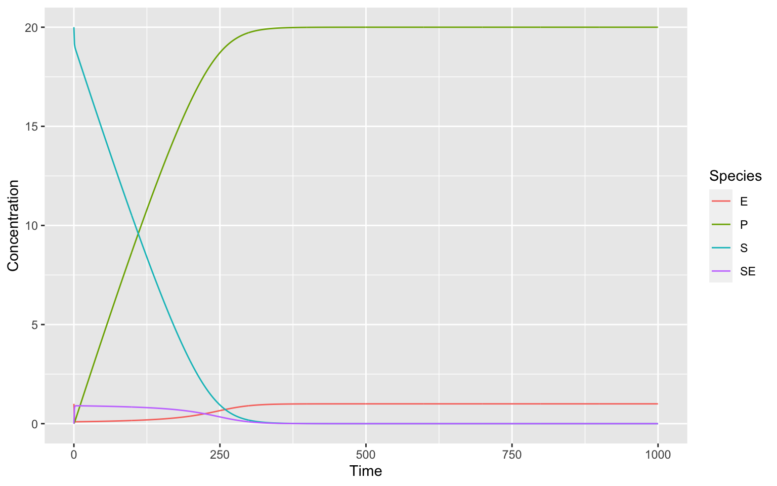
There are two ways of deriving the Michaelis-Menten Kinetics from here. The Quasi-Steady-State Assumption and the Equilibrium approximation. You have to keep in mind, that both of these have underlying assumptions that need not necessarily be true for your model.
Quasi-steady-state Assumption
The approximation taken in this assumption is, that the concentration of the complex is in steady state (at least in the time scale of product formation that we are interested in). This derivation was proposed by Briggs and Heldane 2 and is a bit more intuitive than the original (below).
So, we assume the concentration of the complex does not change over time. \[\frac{d[ES]}{dt} = k_f[S][E] - k_r[SE] - k_{cat}[SE] = 0 \] We can rearrange this to \[ k_f[S][E] = k_r[SE] + k_{cat}[SE] = [SE](k_r + k_{cat})\]
We can see that no enzyme is being destroyed in any process of our model. So we can infer that our total enzyme concentration \(E_0\) does not change over time.
\[ [E_0] = [E] + [ES] = constant \] and from this we get \[ [E] = [E_0]-[ES]\] With this, we can solve our expression
\[k_f[S][E] = [ES](k_r + k_{cat}) \] by inserting it into this formula:
\[k_f[S]*([E_0]-[ES]) = [ES](k_r + k_{cat}) \] \[k_f[S][E_0] - k_f[S][ES] = [ES](k_r + k_{cat}) \] \[k_f[S][E_0] = [ES](k_r + k_{cat} + k_f[S])\] \[[ES] = \frac{k_f[S][E_0]}{k_r + k_{cat} + k_f[S]}\] We can use a trick and multiply \(k_f\) out in the denominator to get rid of \(k_f\) in the numerator \[[ES]= \frac{k_f[S][E_0]}{k_f(\frac{k_r+k_{cat}}{k_f}+[S])}\] \[[ES]= \frac{[S][E_0]}{(\frac{k_r+k_{cat}}{k_f}+[S])}\] Now, to make it nicer to look at, we will define: \[ \frac{k_r + k_{cat}}{k_f} = K_M \] Our equation now looks already very similar to the Michaelis-Menten-Kinetics \[[ES] = \frac{[S][E_0]}{K_M + [S]}\]
What we now want is the velocity of the product formation: \[v = \frac{d[P]}{dt} = k_{cat}[ES] \] We can insert what we derived about the \([ES]\) in the second to last equation: \[ v = k_{cat} * \frac{[S][E_0]}{K_M + [S]} \] Now, we can say, that if all available enzyme was creating the product at the same time (\([E_0] * k_{cat}\)), we would have the maximum velocity (\(V_{max}\)) of this reaction. So we can define:
\[ V_{max} = [E_0]*k_{cat} \]
Finally, when we insert this in our reaction velocity, we get the Michaelis-Menten Reaction kinetics:
\[v = \frac{V_{max}[S]}{K_M + [S]} \]
Equilibrium approximation
Alternatively, we can approximate these kinetics by applying an Equilibrium approximation, where we assume that the substrate is in chemical equilibrium with the complex. This was the original derivation from Leonor Michaelis and Maud Menten. We assume that the forward reaction is equal to the backwards reaction:
\[k_f[S][E] = k_r[SE]\]
The derivation of the Michaelis-Menten kinetics from this is similar to the above derivation (the interpretation of the Michaelis constant is slightly different though), so we will skip that.
Comparing models
Now, we want to show how our Michaelis-Menten-Kinetics work. For this, we will plot the substrate and product concentration of our model next to the substrate and product concentration of a model with built-in Michaelis-Menten-Kinetics that looks like this:
\[ S \rightarrow P \]
We will first save a reference to our current model in a variable to start working on a new model:
manualMM <- getCurrentModel()

newModel()
#> # A COPASI model reference:
#> Model name: "New Model"
#> Number of compartments: 0
#> Number of species: 0
#> Number of reactions: 0
setModelName("Inbuilt Michaelis Menten")
We only need one reaction, but we need to set our rate law to “Michaelis-Menten”.
newReaction("S -> P", fun = "Michaelis-Menten (irreversible)")
#> [1] "(S -> P)"
inbuiltMM <- getCurrentModel()
We need to make sure that our models have the same parameters so that they would behave the same, if they are the same. Let us take a look at the parameters:
getParameters(model = manualMM)
#> # A tibble: 3 × 5
#>   key              name  reaction    value mapping
#>   <chr>            <chr> <chr>       <dbl> <chr>
#> 1 (S + E = SE).k1  k1    S + E = SE    0.1 <NA>
#> 2 (S + E = SE).k2  k2    S + E = SE    0.1 <NA>
#> 3 (SE -> P + E).k1 k1    SE -> P + E   0.1 <NA>
getParameters(model = inbuiltMM)
#> # A tibble: 2 × 5
#>   key         name  reaction value mapping
#>   <chr>       <chr> <chr>    <dbl> <chr>
#> 1 (S -> P).Km Km    S -> P     0.1 <NA>
#> 2 (S -> P).V  V     S -> P     0.1 <NA>
As we can see, our inbuilt reaction still needs some parameters set, to make the models comparable. The \(K_M\) we can easily be set with our formula which was derived earlier:
\[K_M = \frac{k_r + k_{cat}}{k_f} \]
The parameters in our model correspond to (from top to bottom): \(k_f\), \(k_r\), \(k_{cat}\). All of them are 0.1 so for \(K_M\) we get \(K_M = 0.2 / 0.1 = 2\).
Finding the \(v_{max}\) is a bit more tricky. We defined: \[ V_{max} = [E_0]*k_{cat} \]
\(k_{cat}\) is 0.1, as we just found out, but for \(E_0\) we need to take a look at the species in our manual Michaelis Menten Model:
getSpecies(model = manualMM)
#> # A tibble: 4 × 13
#>   key             name  compartment type   unit  initial_concent… initial_number
#>   <chr>           <chr> <chr>       <chr>  <chr>            <dbl>          <dbl>
#> 1 E{compartment}  E     compartment react… mol/l                1        6.02e23
#> 2 S{compartment}  S     compartment react… mol/l               20        1.20e25
#> 3 SE{compartment} SE    compartment react… mol/l                0        0
#> 4 P{compartment}  P     compartment react… mol/l                0        0
#> # … with 6 more variables: concentration <dbl>, number <dbl>, rate <dbl>,
#> #   number_rate <dbl>, initial_expression <chr>, expression <chr>
The total enzyme concentration \(E_0\) is defined as
\[ [E_0] = [E] + [SE] = 1 + 0 = 1\] and it follows for \(V_{max}\) \[ V_{max} = [E_0] * k_{cat} = 1 * 0.1 = 0.1 \] We can set these parameters for our inbuilt Michalis Menten model. Additionally, we set the species starting concentration so that they are the same as for the manual model:
setParameters(model = inbuiltMM, key = parameter(model = inbuiltMM), value = c(2, 0.1))
setSpecies(model = inbuiltMM, key = species(model = inbuiltMM), initial_concentration = c(0,20))
Now, we can run a time course for both models:
manualTC  <- runTimeCourse(duration = 1000, dt = 0.1, model = manualMM)$result
inbuiltTC <- runTimeCourse(duration = 1000, dt = 0.1, model = inbuiltMM)$result
and plot the product and the substrate over time:
ggplot(mapping = aes(x = Time))+
geom_line(data = inbuiltTC, mapping = aes(y = S, color = "Substrate"))+
geom_line(data = inbuiltTC, mapping = aes(y = P, color = "Product")) +
geom_line(data = manualTC, mapping = aes(y = S, color = "Substrate"), linetype = "dotted")+
geom_line(data = manualTC, mapping = aes(y = P, color = "Product"), linetype = "dotted")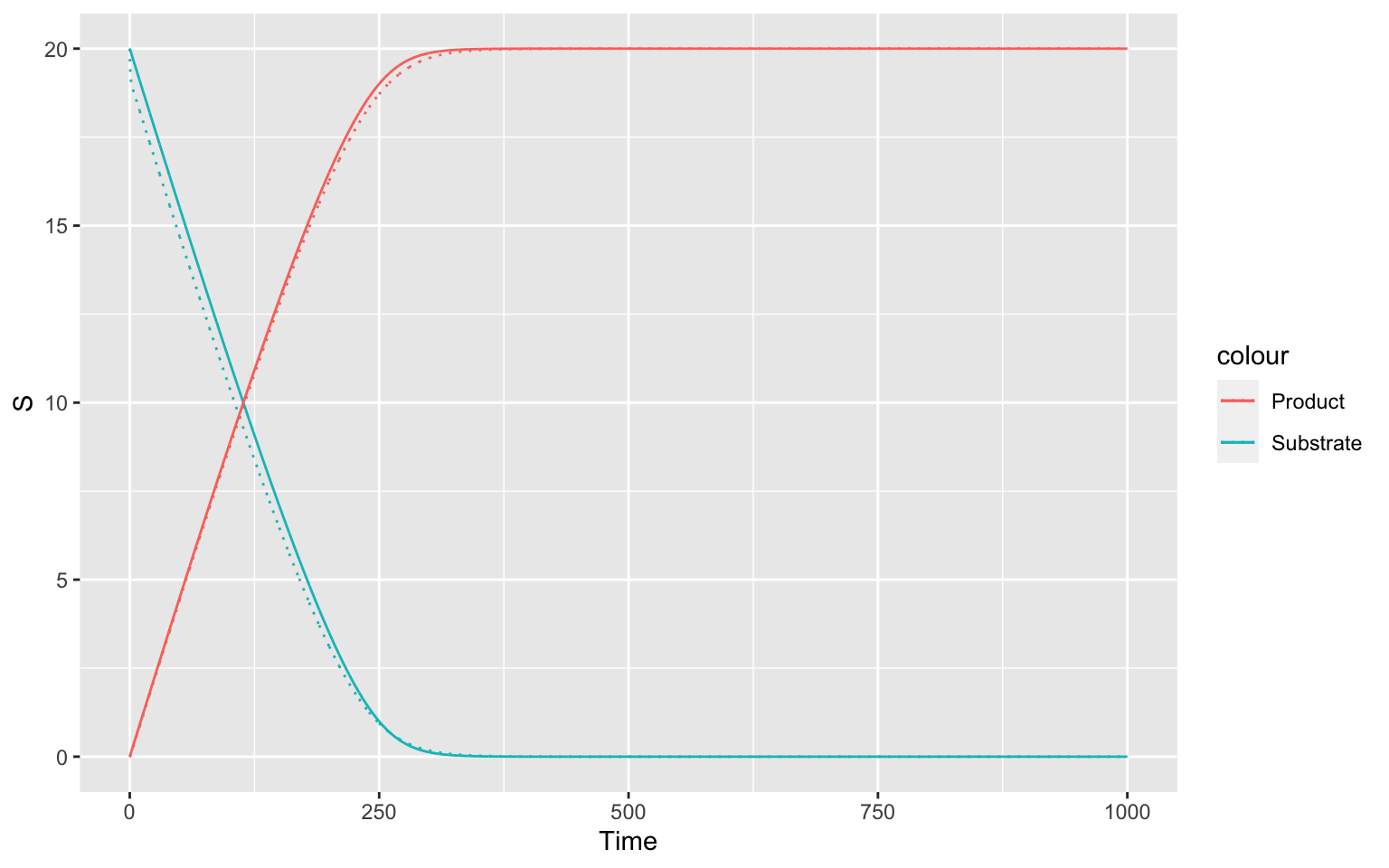 As you can see, the dotted (for manual) and the solid line (for inbuilt)
vary slightly, but they are very similar.
As you can see, the dotted (for manual) and the solid line (for inbuilt)
vary slightly, but they are very similar.
Non-Michaelis-Menten Kinetics
We have seen, that the Michaelis-Menten Kinetics do not apply to every reaction in every model. From the assumptions that are in the Michaelis-Menten Kinetics, we can see which reactions cannot be approximated well with these kinetics:
The Reaction is not catalysed by an enzyme. This seems straightforward, but it is something to keep in mind. You need to have one species in your reaction that is needed for the reaction but does not change during the reaction.
The concentration of the enzyme changes over time. Keep in mind that we assumed that \(E_0\) (the total enzyme concentration) does not change over time. We need that assumption, and if it is not true, our model will not describe reality very well, if we still used Michaelis-Menten Kinetics.
The concentration of the complex is not in steady state / The substrate is not in equilibrium with the complex. This is the basis for the Quasi-Steady-State and Quasi-Equilibrium assumption respectively. If this assumption is not true, we will not be able to model our reaction using Michaelis-Menten-Kinetics.
Our reaction is not \(S + E \rightleftharpoons SE \rightarrow E + P\). Again, this seems really straightforward, but there are a lot of reactions that will not be described with this basis. What would happen, if you needed a helper binding to the enzyme for the substrate to bind? Or if you have two substrates, where one first binds to the enzyme and then the other? Or, very likely, the substrate to product reaction is not irreversible?
What happens if it goes wrong
Let us try and model a few reaction with Michaelis-Menten-Kinetics, where the assumptions needed to apply the kinetics are not met.
Let us start with one, where the equilibrium approximation does not hold:
\[ k_f[S][E] \ne k_r[SE]\]
# not Equilibrium
newModel()
#> # A COPASI model reference:
#> Model name: "New Model"
#> Number of compartments: 0
#> Number of species: 0
#> Number of reactions: 0
setModelName("no Equilibrium")
newReaction("S + E -> SE")
#> [1] "(S + E -> SE)"
newReaction("SE -> P + E")
#> [1] "(SE -> P + E)"

getSpecies()
#> # A tibble: 4 × 13
#>   key             name  compartment type   unit  initial_concent… initial_number
#>   <chr>           <chr> <chr>       <chr>  <chr>            <dbl>          <dbl>
#> 1 E{compartment}  E     compartment react… mol/l                1        6.02e23
#> 2 S{compartment}  S     compartment react… mol/l                1        6.02e23
#> 3 SE{compartment} SE    compartment react… mol/l                1        6.02e23
#> 4 P{compartment}  P     compartment react… mol/l                1        6.02e23
#> # … with 6 more variables: concentration <dbl>, number <dbl>, rate <dbl>,
#> #   number_rate <dbl>, initial_expression <chr>, expression <chr>
getReactions()
#> # A tibble: 2 × 6
#>   key           name        reaction    rate_law                flux number_flux
#>   <chr>         <chr>       <chr>       <chr>                  <dbl>       <dbl>
#> 1 (S + E -> SE) S + E -> SE S + E -> SE FunctionDB.Functions[…     0           0
#> 2 (SE -> P + E) SE -> P + E SE -> P + E FunctionDB.Functions[…     0           0

setSpecies(key = species(), initial_concentration = c(1,20,0,0))

noEqu <- getCurrentModel()
And we can have another one, where the concentration of the enzyme changes over time:
# Enzyme changes
newModel()
#> # A COPASI model reference:
#> Model name: "New Model"
#> Number of compartments: 0
#> Number of species: 0
#> Number of reactions: 0
setModelName("Changing Enzyme")
newReaction("S + E = SE")
#> [1] "(S + E = SE)"
newReaction("SE -> P + E")
#> [1] "(SE -> P + E)"
newReaction("E ->")
#> [1] "(E ->)"

getSpecies()
#> # A tibble: 4 × 13
#>   key             name  compartment type   unit  initial_concent… initial_number
#>   <chr>           <chr> <chr>       <chr>  <chr>            <dbl>          <dbl>
#> 1 E{compartment}  E     compartment react… mol/l                1        6.02e23
#> 2 S{compartment}  S     compartment react… mol/l                1        6.02e23
#> 3 SE{compartment} SE    compartment react… mol/l                1        6.02e23
#> 4 P{compartment}  P     compartment react… mol/l                1        6.02e23
#> # … with 6 more variables: concentration <dbl>, number <dbl>, rate <dbl>,
#> #   number_rate <dbl>, initial_expression <chr>, expression <chr>
setSpecies(key = species(), initial_concentration = c(1,20,0,0))

getParameters()
#> # A tibble: 4 × 5
#>   key              name  reaction    value mapping
#>   <chr>            <chr> <chr>       <dbl> <chr>
#> 1 (S + E = SE).k1  k1    S + E = SE    0.1 <NA>
#> 2 (S + E = SE).k2  k2    S + E = SE    0.1 <NA>
#> 3 (SE -> P + E).k1 k1    SE -> P + E   0.1 <NA>
#> 4 (E ->).k1        k1    E ->          0.1 <NA>
setParameters(key = parameter(), value = c(0.1, 0.1, 0.1, 0.2))

EnzCh <- getCurrentModel()
Both of these “true” reactions would be modelled with the same Michaelis-Menten-Kinetics so let’s see how that holds up:
noEquTC <- runTimeCourse(model = noEqu, duration = 1000, dt = 0.1)$result
EnzChTC <- runTimeCourse(model = EnzCh, duration = 1000, dt = 0.1)$result

ggplot(mapping = aes(x = Time))+
  geom_line(data = inbuiltTC, mapping = aes(y = S, color = "Substrate"))+
  geom_line(data = inbuiltTC, mapping = aes(y = P, color = "Product"))+
  geom_line(data = noEquTC,   mapping = aes(y = S, color = "Substrate"), linetype = "dashed")+
  geom_line(data = noEquTC,   mapping = aes(y = P, color = "Product"), linetype = "dashed")+
  geom_line(data = EnzChTC,   mapping = aes(y = S, color = "Substrate"), linetype = "dotted")+
  geom_line(data = EnzChTC,  mapping = aes(y = P, color = "Product"), linetype = "dotted")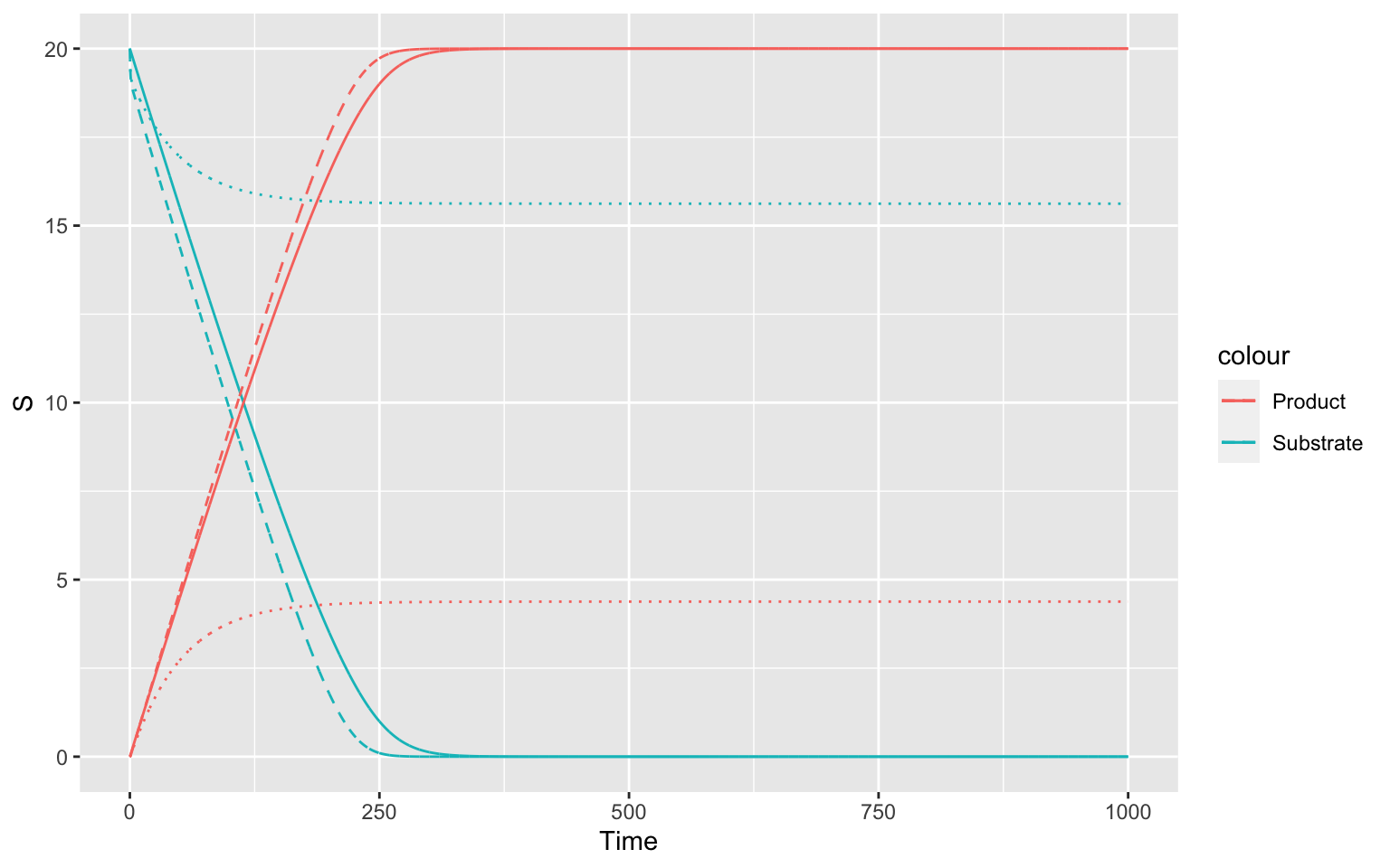
The dashed line (where the equilibrium approximation is not true) and especially the dotted line (where the amount of enzyme changes over time) differ significantly from the inbuilt kinetics.
More complicated kinetics
We can expand our reaction kinetics in a lot of ways. We will now find the “Michaelis-Menten-Like” kinetics for the following reaction, where the product formation is reversible:
\[ S + E \rightleftharpoons SE \rightleftharpoons E + P \]
with parameters \(k_f\) and \(k_r\) for the first reaction and \(k_F\) and \(k_R\) for the second reaction.
Our differential equations will now look the following:
\[\frac{d[S]}{dt} = - k_f[S][E] + k_r[SE]\] \[\frac{d[E]}{dt} = -k_f[S][E] + k_r[SE] + k_{F}[SE] - k_R[E][P]\] \[\frac{d[ES]}{dt} = k_f[S][E] - k_r[SE] - k_{F}[SE] + k_R[E][P] \] \[\frac{d[P]}{dt} = k_{F}[SE] - k_R[E][P]\]
We will use the equilibrium assumption, where we assume that the first forward reaction is equal to the first backward reaction:
\[k_f[S][E] = k_r[SE]\] We can again use \(E_0 = [E]+[SE] \rightarrow [E] = [E_0] - [SE]\): \[ k_f[S]([E_0]-[SE]) = k_r[SE]\] and move our equations around so we will have a formula for \([SE]\): \[k_f[S][E_0]-k_f[S][SE] = k_r[SE]\] \[\hookrightarrow [SE] = \frac{k_f[S][E_0]}{k_r + k_f[S]}\] We can again multiply out k_f: \[[SE] = \frac{[S][E_0]}{\frac{k_r}{k_f}+[S]}\] Now, we want to know the velocity of the product formation, where the differential equation is: \[v = \frac{d[P]}{dt} = k_{F}[SE] - k_R[E][P]\] We can put in what we found out for the concentration of the complex: \[ v = k_F\frac{[S][E_0]}{\frac{k_r}{k_f}+[S]} -k_R[E][P]\] and now, we have our reaction velocity for reversible Michaelis-Menten Kinetics.
What to learn from that
Michaelis-Menten Kinetics are a beautiful and relatively intuitive approximation of enzyme kinetics. But you have to keep in mind, that every approximation is built on assumptions and you have to check carefully if those assumptions are true for the specific reaction in your model. There are a lot of other kinetics possible for the interaction of species in a model and it is always useful to understand what they are doing and why. This way, your model will be the best it can be!
References
L. Menten, M. Michaelis, Die Kinetik der Invertinwirkung, Biochem Z49 (333-369) (1913) 5↩︎
George Edward Briggs, John Burdon Sanderson Haldane; A Note on the Kinetics of Enzyme Action. Biochem J 1 January 1925; 19 (2): 338–339. doi: https://doi.org/10.1042/bj0190338↩︎